Rethinking Robot Modeling and Representations
An overview of Neural Jacobian Field, an architecture that autonomously learns to represent, model, and control robots in a general-purpose way.
Advised by Vincent Sitzmann, MIT CSAIL
Was Du ererbt von Deinen Vätern hast, erwirb es, um es zu besitzen. (Goethe)
TL;DR
We present a solution that learns a controllable 3D model of any robot, from vision alone. This includes robots that were previously intractable to model by experts. [Code] [Project Page] [Video]
Motivation
Have you ever wondered why robots today are so costly? Why are they almost always made of rigidly jointed segments? What if I tell you that this is largely due to challenges in building digital models of these robots, rather than hardware challenges?
What even is a robot anyways?
Let’s take a step back and think about what a robot even is. Slapping a few motors on an IKEA Lamp with a Raspberry Pi, we have mechanical system that we can command to move around in space. Is that a robot? (This turns out to be a rather difficult question). We would argue that if a machine is capable of solving the physical task you are interested in, then it is a valid robot.
The minimum requirement – the ability to control
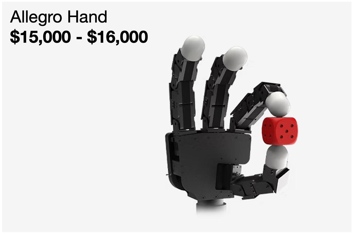
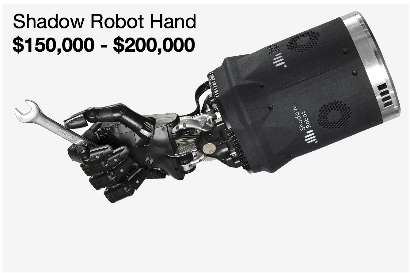
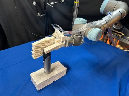
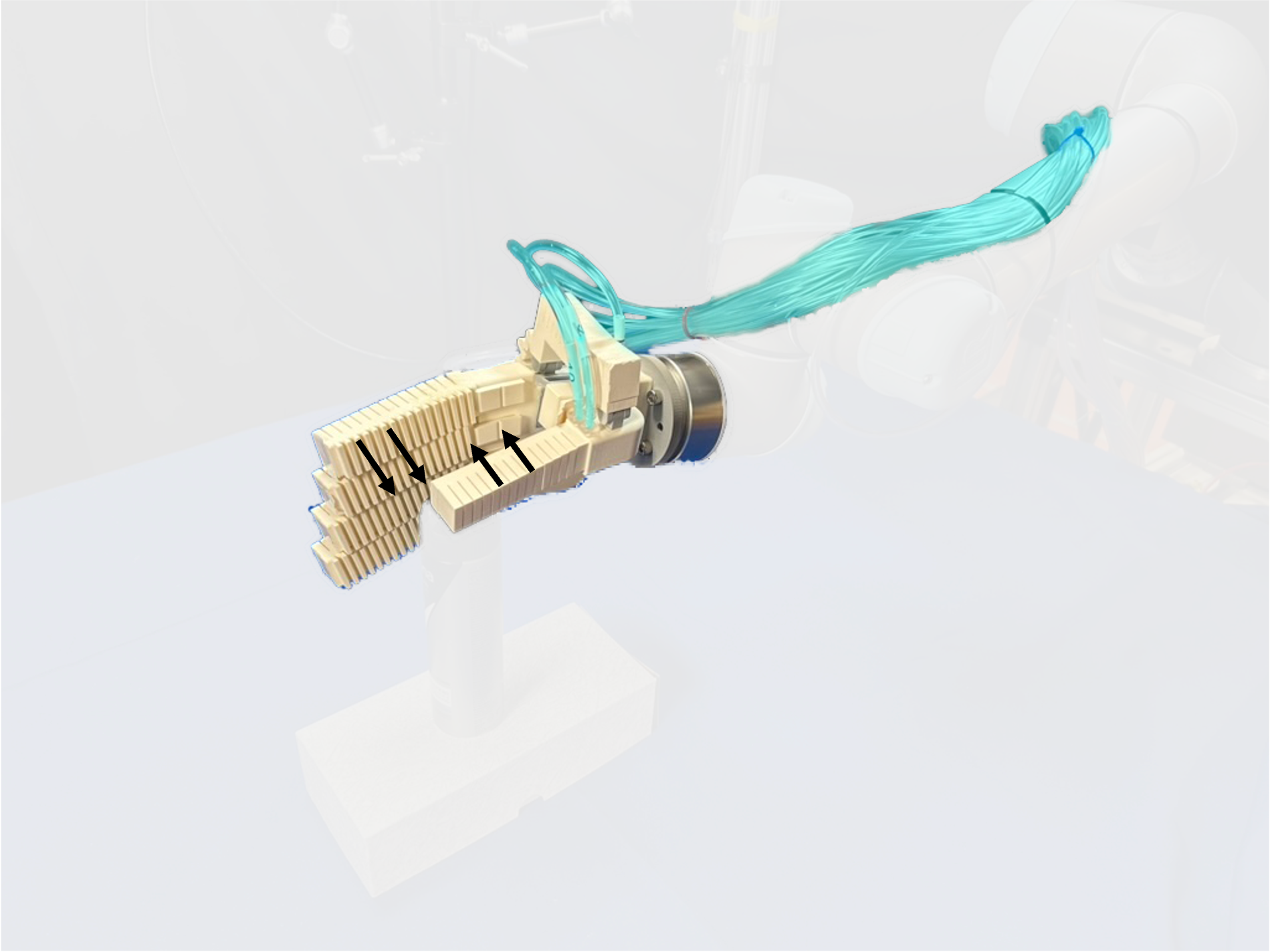
Perhaps a valid definition of a robot includes a criterion of controllability. We need to be able to control the robot to call it one. That’s why many people wouldn’t call the motorized IKEA lamp a robot – today we do not have an algorithm that can control it effectively. Next, we have a second robot – a pneumatic hand (left figure) – that shares the same property as our IKEA robot. Namely, today this robot is also not controllable.
The central question of control is: given a desired motion for my robot hand, what change of command should I send? (right figure)
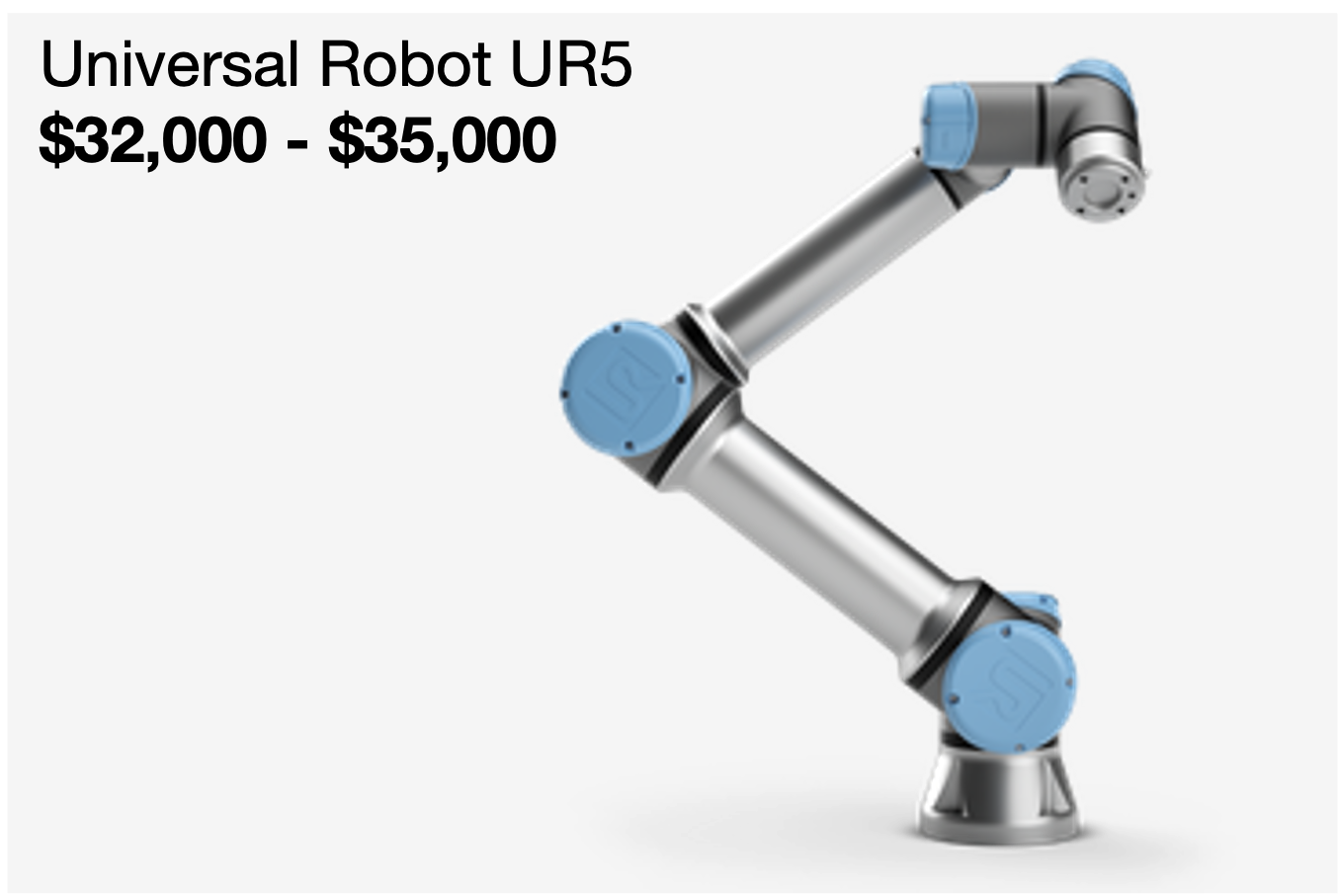
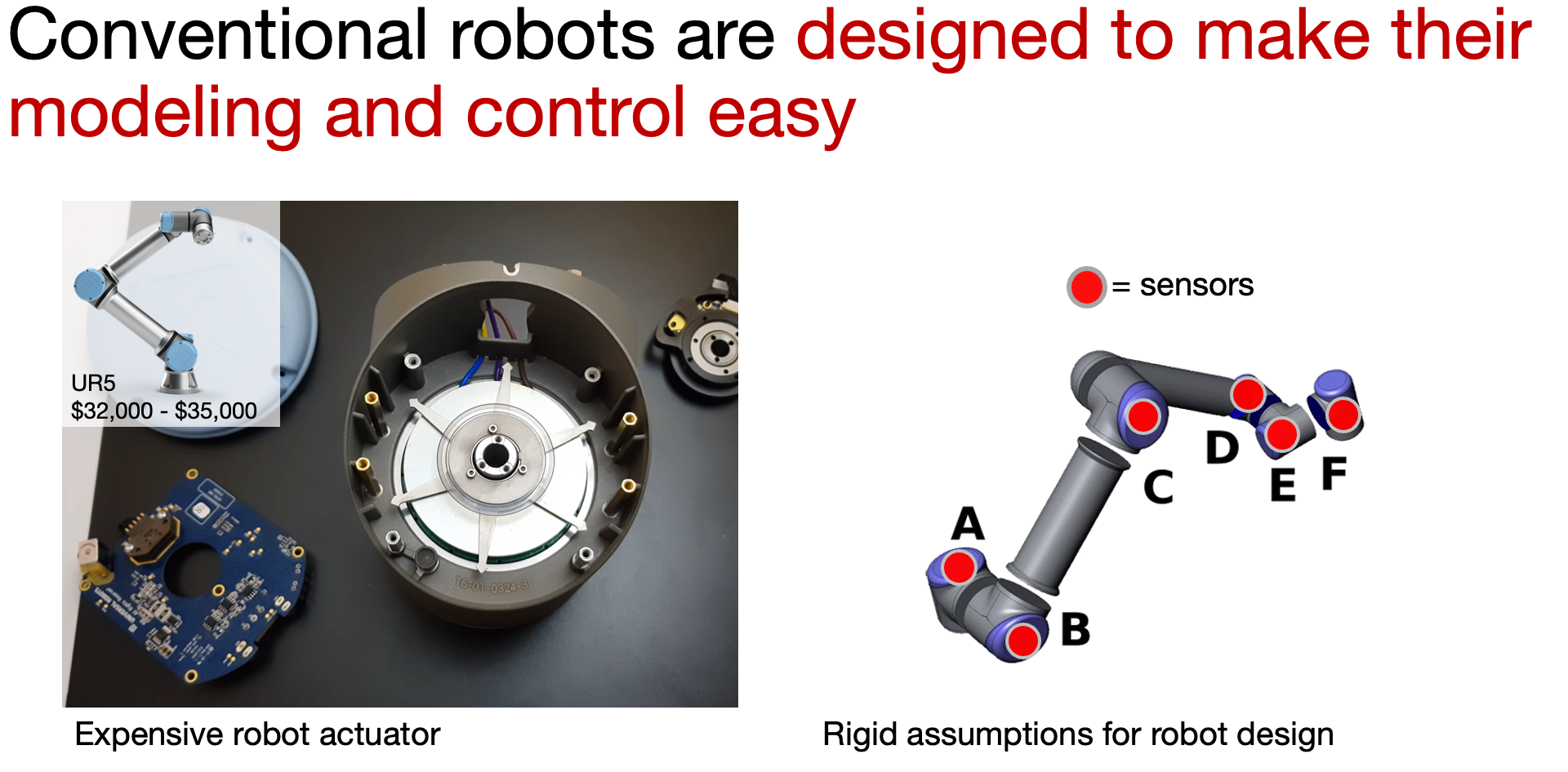
Today, most robots look like the UR5 below. These robots inherit a special class of sensors and morphologies for making them controllable.
Why is the past solution no longer adequate
The way we have approached this problem in the past has reached a ceiling. It turns out that past solutions cannot model the robots above, since these robots lack sensory measurements and experience deformations.
This is a part of why robotic automation today remains costly. We have cheaper hardware designs that can still perform the same physical tasks, but the conventional software does not support these hardwares. As a result, our robots are often over-engineered to compensate the software limitations.
For mechanical systems like airplanes and trains, it makes sense to design special-purpose sensors that measure the almost exact states. These sensory measurements typically support a model that suits the problem domains. This is because the application domain for these control problem requires extreme modeling accuracy and reaction times.
However, the conventional modeling spirit doesn’t seem suitable for the coming age of general-purpose robotics. It assumes that the environment and the robot are modeled separately. It assumes that scissors and screwdrivers arrive with internal sensors reporting their states. It assumes that robots and the world have a fixed form of morphology and physical properties.
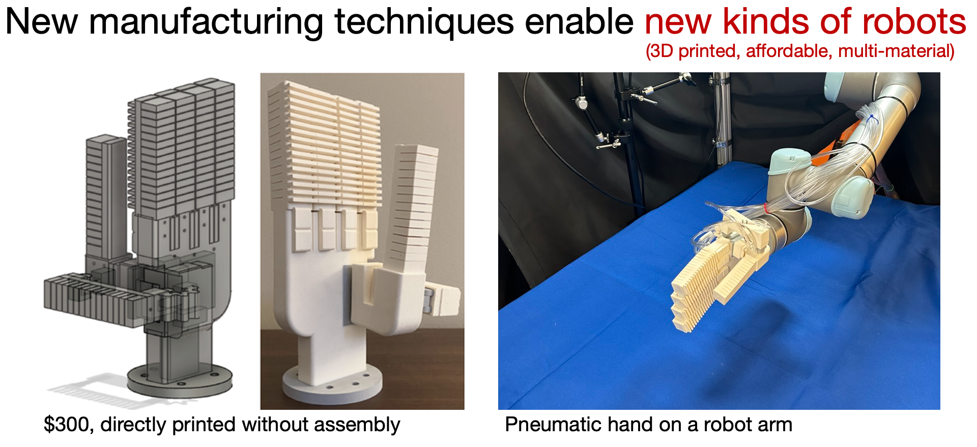
A new spirit forward
A new modeling spirit is needed for more accessible robotic automation. One that integrates recent advances in computational perception, with powerful tools from machine learning, mechanics, and control. One that lifts the modeling assumptions to a level suitable for general-purpose robotics. One that requires new algorithms that go beyond precise sensor feedback and idealized dynamics.
Achieving this vision carries values to our society. Imprecise, flexible, and unconventional robots
Jacobian Fields
Jacobian Fields is an approach that aims to address problems we posed above. The core idea is to spatialize the conventional end-effector Jacobian in robot dynamics, and compute a field of such operators in the Euclidean space. We encourage the readers to refer to Chapter 5 of Modern Robotics
The Body Jacobian
Look at this 2D robot arm! For any spatial point $(x, y)$ on the robot. Given a small variation of the joint angles $\delta q$, we can find Jacobian of the following form
\[\begin{bmatrix} \delta {x} \\ \delta {y} \end{bmatrix} = J(q) \begin{bmatrix} \delta {q}_1 \\ \delta {q}_2 \end{bmatrix}.\]For more formalism and details, please check out our appendix on the system Jacobian.
Spatialization of Jacobian
We can spatialize our Jacobian. This lifts our representation from reduced or minimal coordinates to the Euclidean space and draws deep connections with recent advances in computational perception.
To formally describe this idea using continuum mechanics
Now, we have the spatial system Jacobian as follows
\[\begin{equation} \mathbf{x}^{+} = \mathbf{\phi}(\mathbf{x} | \bar{\mathbf{q}} , \bar{\mathbf{u}}) + \frac{\partial \mathbf{\phi}(\mathbf{x} | \mathbf{q}, \mathbf{u})}{\partial \mathbf{u}} \bigg\rvert_{\bar{\mathbf{q}}, \bar{\mathbf{u}}} \delta \mathbf{u}. \end{equation}\]The spatial differential quantity $\frac{\partial \mathbf{\phi}(\cdot | \mathbf{q}, \mathbf{u})}{\partial \mathbf{u}} $ is precisely the Jacobian Field that we are interested in learning and measuring from perceptual observations.
Learning and measuring Jacobian Fields from perceptual inputs
We now use a simple 2D example to illustrate the idea of Jacobian Fields. Please check out the pytorch implementation of tutorial 1 to reproduce our results in this section.
2D Pusher Environment. The environment contains a spherical robotic pusher. The robot can move freely in 2D space and is steered by a 2D velocity command $\delta u \triangleq (x, y)$, where $x, y \in \mathbb{R}$.
Training Samples Illustration. We now illustrate the two training samples in our dataset, moving down and to the right. The following same-row videos might become async due to HTML rendering.
How can we learn Jacobian Fields from visual perception to “explain away” our observed optical flow motions? We first find that our solid domain here, $\Omega^{t}$, equates the pixel space $\mathbb{R}^{H\times W}$ that we perceive. This is not always the case, as the 3D world induces a projection process to imaging devices and contains occluding and refracting surfaces.
We use a standard fully convolutional network (UNet
Given data pair $(I, I^+, \delta u)$, we can set up the following learning problem
\[\begin{equation} \arg\min_{\theta} \ \left\lVert J_\theta \big(x \mid I \big)^\top \delta u - V \big(x \mid I, I^+ \big) \right\rVert, \end{equation}\]where $V$ is the optical flow field computed by a state-of-the-art approach (e.g., RAFT
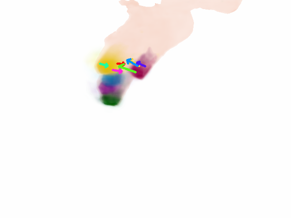
Visualizing the learned Jacobian Fields
Training till convergence, using just two samples, our Jacobian Field is able to explain unseen image observations and command directions. We will soon delve deeper into the physics of why Jacobian Fields can generalize here. The short answers are invariance, locality, and compositionality of the Jacobians.
How are we visualizing the Jacobians? We simply assign color component to each channel of the Jacobian field. For every spatial coordinate, we compute the norm over spatial channel to derive the total spatial sensitivity vector of the Jacobian. Please check out the pytorch implementation of tutorial 1 to reproduce our results in this section.
A second example in 2D
Let’s train our Jacobian Fields in another environment, but this time more compositional and dexterous! Please check out the pytorch implementation of tutorial 2 to reproduce our results in this section.
Finger Environment. The environment contains a 2 degrees-of-freedom robot finger. The robot finger is commanded by a 2D joint velocity command $\delta u \triangleq (u_1, u_2)$, where $u_1, u_2 \in \mathbb{R}$ control the rotations of each motor respectively.
The same idea successfully disentangles the different spatial components of motion.
Unified representation with environment variables
The idea of Jacobian Fields extends to capture dynamics with environment variables, such as contacts with continuum bodies.
Real-world examples
Remarkably, the same idea extends to the real world and to 3D. By incorporating the image formation model and neural rendering, we can use optical flows observed with 2D cameras to explain away the underlying flow field in the 3D world.
Here are a few examples, please check out the pytorch implementation of tutorial 3 and tutorial 4 to reproduce our results in this section.
Controlling the robot with Jacobian Fields
After training, Jacobian Fields can be used for inverse dynamics. We have new upcoming results showing that a flow planner can be flexibly integrated into the approach, stay tuned!
For now, let’s illustrate the idea by just using a keypoint trajectory and a model-predictive controller.
Connections with invariance, locality, and compositionality
1. Linearity from Local Theory of Smoothing
We model differential kinematics by linearizing the system dynamics, which represents 3D motion fields induced by small control commands $\delta u$. In this regime, it is well-known that the 3D motion $\delta x$ of robot 3D points can be described by the space Jacobian and is thus a linear function of control commands, i.e. $\alpha \delta x = \frac{\partial f}{\partial u} (\alpha \delta u)$.
This is powerful, as completely specifying the system dynamics for a particular configuration $u’$ requires only $n \times 3$ linearly independent observations of pairs of control commands and induced scene flow, as this fully constrains the space Jacobian for a given configuration for a system with $n$ control channels.
For instance, one need not observe the motions for both $-\delta u$ and $\alpha \delta u$; it suffices to observe one of them. Similarly, one need not observe $\delta u$ and a scalar multiple $\alpha \delta u$; again, one of them in the training set suffices. This is in stark contrast to parameterizing $f$ as a neural network that directly predicts scene flow given an image and a robot command since the neural network does not model these symmetries and will thus require orders of magnitude more motion observations to adequately model the system dynamics.
2. Spatial Locality of Mechanical Systems
Robot commands often result in highly localized spatial motion. Consider the two finger example we experiment with above, within a “rigid” segment, the Jacobian tensors are locally smooth as we spatially perturb the coordinate value.
3. Spatial Compositionality of Mechanical Systems
Robot commands often result in spatial motions composed by the influences of individual command channels. The two linkage robot finger we experiment with above is a great example. For a point inside the second segment, its motion is the integral over individual command channels in the Jacobian tensor field. Indeed, our predicted 2D motion is the summation over two Jacobian channels.
Project Website
For more information about our project, please check out our project website. Feel free to email sizheli@mit.edu or create an issue on our GitHub repo for any questions!
Related Works
For a comprehensive discussion of related works, please refer to Section 6 of our Nature paper.
Acknowledgement
Sizhe Lester Li is presenting on behalf of the team in the 2025 paper “Controlling diverse robots by inferring Jacobian fields with deep networks.” We would like to thank Isabella Yu for the visualizations of two-finger Jacobian Fields.
Bibtex
If you find this blog helpful, please consider citing our work
@Article{Li2025,
author={Li, Sizhe Lester
and Zhang, Annan
and Chen, Boyuan
and Matusik, Hanna
and Liu, Chao
and Rus, Daniela
and Sitzmann, Vincent},
title={Controlling diverse robots by inferring Jacobian fields with deep networks},
journal={Nature},
year={2025},
month={Jun},
day={25},
issn={1476-4687},
doi={10.1038/s41586-025-09170-0},
url={https://doi.org/10.1038/s41586-025-09170-0}
}
Details on System Jacobian
We first derive the conventional system Jacobian
Local linearization of $\mathbf{f}$ around the nominal point $(\bar{\mathbf{q}}, \bar{\mathbf{u}})$ yields
\[\begin{equation} \mathbf{q}^{+} = \mathbf{f}(\bar{\mathbf{q}}, \bar{\mathbf{u}}) + \frac{\partial \mathbf{f}(\mathbf{q}, \mathbf{u})}{\partial \mathbf{u}} \bigg\rvert_{\bar{\mathbf{q}}, \bar{\mathbf{u}}} \delta \mathbf{u}. \end{equation}\]Here, $\mathbf{J}(\mathbf{q}, \mathbf{u}) = \frac{\partial \mathbf{f}(\mathbf{q}, \mathbf{u})}{\partial \mathbf{u}}$ is known as the system Jacobian, the matrix that relates a change of command $\mathbf{u}$ to the change of state $\mathbf{q}$.
Conventionally, modeling a robotic system involves experts designing a state vector $\mathbf{q}$ that completely defines the robot state, and then embedding sensors to measure each of these state variables. For example, the piece-wise-rigid morphology of conventional robotic systems means that the set of all joint angles is a full state description, and these are conventionally measured by an angular sensor in each joint.
However, these design decisions are difficult to apply to soft robots, and more broadly, to mechanical systems whose coordinates cannot be well-defined or sensorized. Here are a few examples
- Soft and Bio-inspired Robots. Instead of discrete joints, large parts of the robot might deform. Embedding sensors to measure the continuous state of a deformable system is difficult, both because there is no canonical choice for sensors universally compatible with different robots and because their placement and installation are challenging.
- Designing the state itself is challenging. In contrast to a piece-wise rigid robot, where the state vector can be a finite-dimensional concatenation of joint angles, the state of a deformable robot is infinite-dimensional due to continuous deformations.
- Contacts, appendages, wear-and-tear can alter the “coordinate system.” Grasping on a screwdriver, the notion of the robotic system extends to the appendage. From an engineering standpoint, it is a bit odd to expect that screwdrivers and scissors arrive with sensors reporting their internal states.
- Multi-sensory integration requires spatialization. Perceptual signals – visual, tactile, or auditory – reveal the same reality of the physical world precisely in the spatial sense. Traditional expert-designed coordinate systems, hand-crafted on a per-robot basis, do not directly present a general solution to integrating different sensory measurements.